The variational perspective formulates diffusion models as latent variable models (LVMs) trained by maximizing the evidence lower bound (ELBO). However, standard derivations of the diffusion ELBO often rely on lengthy algebra manipulations to arrive at the final objective function. Why do we go through the trouble of transforming a simple expectation into a complex sum of KL divergences? This post uncovers the statistical motivation behind this derivation: variance reduction.

A Quick Refresher on Latent Variable Models

In a latent variable model (LVM), we assume the observed data is generated by an unobserved latent factor . The process is defined by a prior and a likelihood . To train a model to fit the data, we aim to maximize the marginal log-likelihood:

The Problem: Computing this expectation directly is intractable. If we try to estimate it via Monte Carlo sampling (), the variance is explodingly high because for high-dimensional data, is effectively zero for almost all sampled from the prior.

The Evidence Lower Bound (ELBO)

To solve this variance issue, we use importance sampling: introduce an approximate posterior , referred to as the proposal distribution, that focuses sampling on regions where the likelihood is non-negligible. This yields the tractable evidence lower bound (ELBO):

Maximizing tightens the lower bound on the log-likelihood . The practical benefit is that by proposing over likely latents via , the variance of the estimator is significantly lower than naive sampling, making the Monte Carlo estimate tractable.

Diffusion Models as Latent Variable Models

Diffusion models are LVMs where the observed data is and the latent is . The data distribution is defined by a fixed forward process that progressively adds noise, forming a Markov chain factorized as:

By the end of this process, is almost pure noise (typically standard Gaussian). To generate samples, we need to run this process in reverse:

The true prior and the true reverse process are intractable. Instead, we fix some approximate prior and learn an approximate reverse process . This lets us approximate with defined as:

The Diffusion Loss

Substituting the forward and backward processes into the negative ELBO yields the diffusion loss . Standard derivations (Lilian Weng, Ho et al. 2020, Sohl-Dickstein et al. 2015) rewrite this loss as a sum of KL divergences:

Key steps:

• Eq (i) is a clever application of Bayes’ rule:
• Eq (ii) considers the telescoping sum .
• Eq (iii) uses law of total expectation. For example, the first expectation can be decomposed as:

But Why?

Often by design, these are KL divergences between Gaussian distributions, for which closed-form solutions exist. But in line 2 of the loss derivation, every term can already be computed. Why go through this algebra to express the objective as a sum of KL divergences?

Surprisingly, most popular treatments of diffusion models present this derivation without explaining its purpose. The only place I have seen it mentioned at all is a single sentence in the DDPM paper (Ho et al. 2020). This post aims to fill that gap.

The Hidden Variance Reduction

The derivation is motivated by a technique widely known in Monte Carlo literature as Rao-Blackwellization. By analytically computing the KL divergence, we reduce the variance of the loss estimator compared to a naive Monte Carlo approximation.

(Note: The classical Rao-Blackwell theorem concerns sufficient statistics, but in Monte Carlo the term “Rao-Blackwellization” is used more broadly for replacing sampling with analytic conditional expectations.)

Variance Reduction by Conditioning

Theorem (Rao-Blackwellization for Monte Carlo). Let be random variables and suppose we want to estimate . Define . Consider two estimators using i.i.d. samples:

1. Monte Carlo: where .
2. Rao-Blackwellized: where .

Then:

1. Both estimators are unbiased: .
2. The Rao-Blackwellized estimator has lower variance: .
3. Equality holds if and only if does not depend on (almost surely).

Proof. (Unbiasedness) By linearity of expectation:

For the second estimator, the law of iterated expectations gives:

(Variance Comparison) Since the samples are i.i.d., we have and . It suffices to show .

By the law of total variance:

Dividing both sides by , we get . Equality holds if and only if (almost surely), which occurs precisely when does not depend on .

Application to Diffusion Models

Let’s apply this theorem to the diffusion loss, using as an example. We wish to estimate:

Setting , , and , the theorem gives us two estimators using i.i.d. samples:

Naive Monte Carlo: Sample for and compute:

Rao-Blackwellized: Sample for and analytically compute the conditional expectation:

The theorem tells us both estimators are unbiased, but the Rao-Blackwellized version has strictly lower variance (since depends on ).

The Rao-Blackwellized version is precisely the KL divergence formulation derived above! By reducing the variance of our loss estimator, we obtain more reliable gradient estimates during training. Lower variance gradients mean that each training step provides a more consistent signal about which direction to update the parameters, leading to more stable optimization and potentially faster convergence.

Experiments

To empirically validate this variance reduction benefit, we trained diffusion models on the “Two Moons” dataset and compared two loss formulations:

• Monte Carlo (MC): where
• Rao-Blackwellized (RB): where

The first experiment examines training dynamics and generation quality, confirming that while both losses can train diffusion models, the RB formulation offers practical advantages. The second experiment directly measures the variance reduction across diffusion timesteps throughout training.

Training Dynamics

Two diffusion models with identical architectures were trained: one using the RB loss and another using the MC loss.

The generated samples at different training steps reveal the difference:

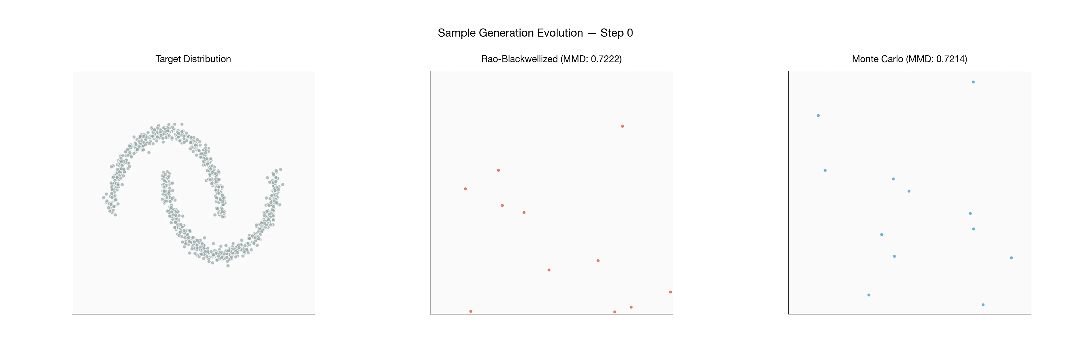
The RB model forms the two moons shape much earlier, and the final converged model seems to generate noticeably better samples. The training loss and sample quality curves confirm this observation:

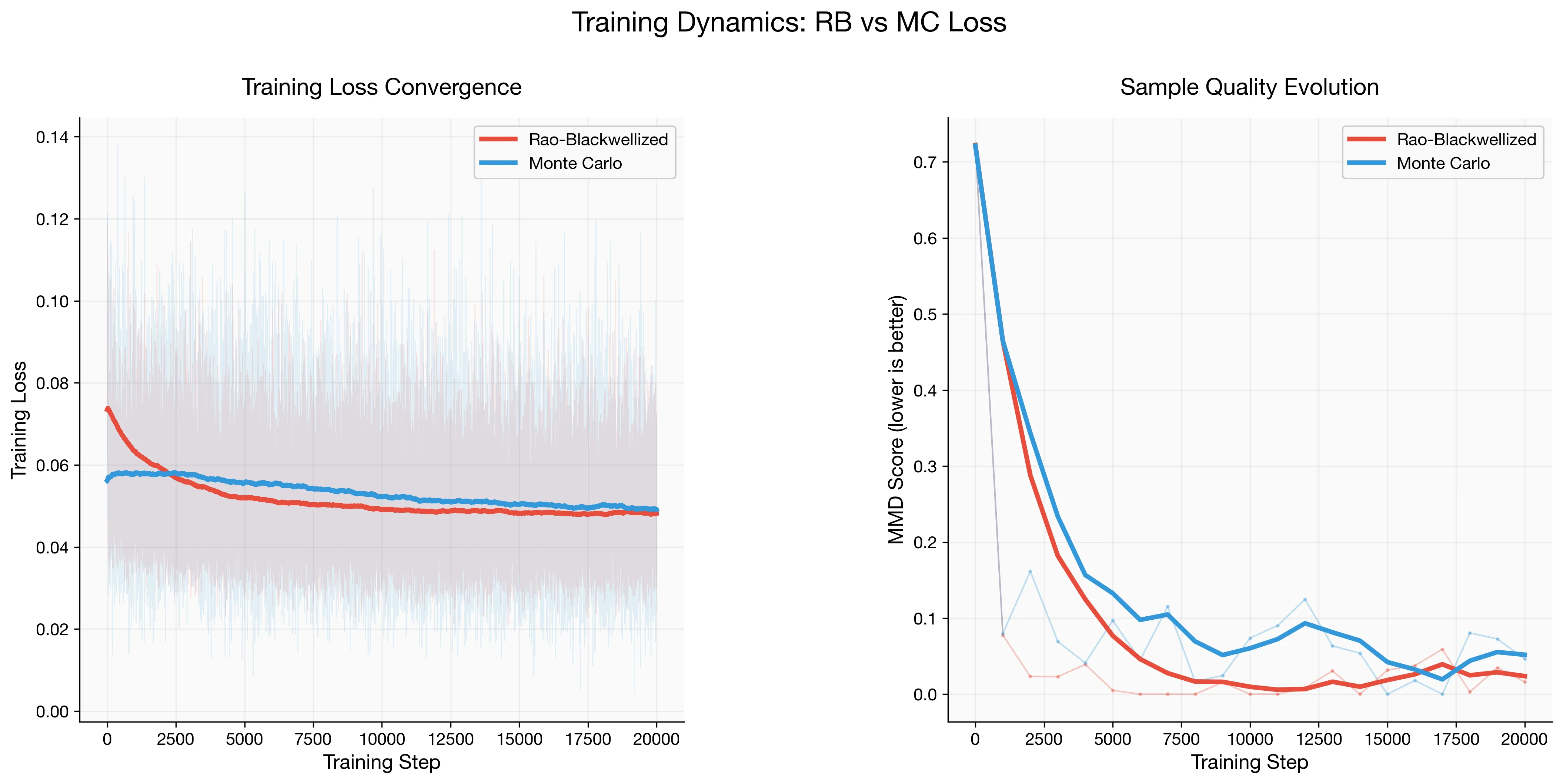
The RB model’s loss decays faster and remains consistently lower throughout training. Measuring sample quality via maximum mean discrepancy (MMD, lower is better), the RB model converges faster and achieves superior sample quality.

Variance Evolution

To directly verify the variance reduction, we trained a single diffusion model and tracked the empirical variance of both loss estimators across all diffusion timesteps throughout training. At regular intervals during training, we:

1. For each timestep , computed both and using a single sample ()
2. Estimated the variance of each estimator by repeating this process multiple times

The results are visualized below:

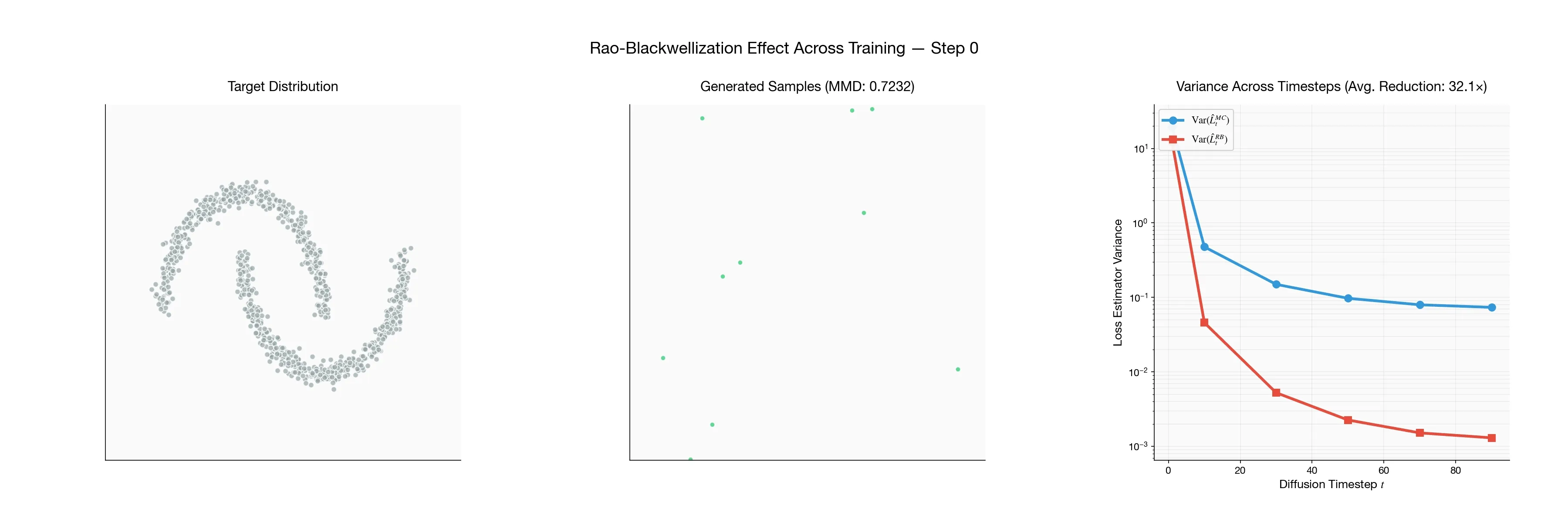
The RB estimator consistently exhibits variance on the order of lower than the MC estimator across all diffusion timesteps . It is surprising that despite this dramatic variance difference, the MC model still produces reasonable results. Notably, the shape of the variance curves remains remarkably consistent throughout training, suggesting that the variance reduction benefit is stable across the optimization trajectory.

Conclusion

The standard derivation of diffusion loss as a sum of KL divergences is not merely algebraic convenience—it is motivated by Rao-Blackwellization, a fundamental variance reduction technique. The algebraic manipulation allows us to reduce loss estimator variance without introducing bias.

Our experiments confirm this matters in practice: the variance reduction ( lower) of the Rao-Blackwellized loss leads to faster convergence, lower final loss, and better sample quality. Surprisingly, the naive Monte Carlo approach still produces reasonable results.